Many of today’s designs are “smart” devices that require high-frequency components and must incorporate RF elements to operate properly. Creating an RF schematic and simulating the RF components is crucial to the success of the design as impedances must be carefully matched. AWR allows you to quickly setup an RF schematic for simulation.
This quick how-to will provide step-by-step instructions on how to create an RF schematic for simulation in AWR Design Environment.
How-To Video
 Open in New Window
Creating an RF Schematic
Step 1: Open a blank project in AWR Design Environment.
Step 2: Select Project > Add Schematic > New Schematic from the menu.
Note: Additional options exist to create schematics.
- Hover over the Project tab to open it.
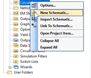
- Right-click Circuit Schematics and select New Schematic.
A schematic can also be created from the toolbar.
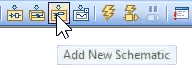
- Select the New Schematic button from the toolbar.
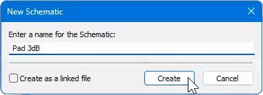
Step 3: Name the schematic Pad 3dB and click Create.
Note: If the name of the schematic is changed in the design, anything that links to the schematic such as graphs will sync automatically.
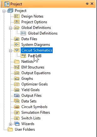
Step 4: Hover over the Project tab to open the Project panel. The schematic has been added under Circuit Schematics.
Adding Components to the Schematic
Step 5: Hover over the Elements tab to open the Elements panel.
Step 6: Expand Lumped Element. Select Resistor.
Note: The Lumped Elements category is where passive components such as resistors and capacitors can be placed from.
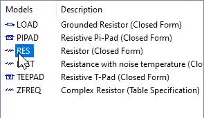
Step 7: Click and hold RES on the element list to place a resistor.
Step 8: Drag your mouse into the schematic and release to attach the resistor to your cursor.
Note: Move the mouse around the canvas to choose the component location. Right-click to rotate. Right-click while holding Shift to flip vertically. Right-click while holding CTRL to flip horizontally.
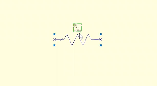
Step 9: Click to place the resistor.
Step 10: Click to select the placed resistor. Press CTRL-C on the keyboard to copy.
Step 11: Press CTRL-V to paste. A new resistor is attached to your cursor.
Step 12: Right-click to rotate and left-click to place the new resistor.
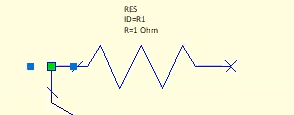
Note: A green square indicates that the components are connected. An “x” indicates no connection.
Step 13: Click and drag to move the resistor. A wire is added automatically.
Note: The resistor can be moved anywhere in the canvas and remain connected.
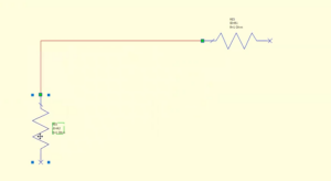
To disconnect a component, hold CTRL, then click and drag it.
To wire distant components, hover over the desired terminal, click once, and click again at the destination terminal.
Step 14: With the resistor selected, press CTRL-C and CTRL-V to copy and paste.
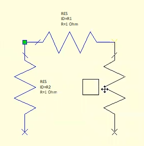
Step 15: Flip the resistor left to right by holding CTRL and right-clicking. Click to place a new resistor on the right side of the original resistor.
Adding a Ground to the Schematic
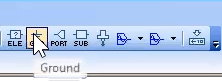
Step 16: Select the GND symbol from the toolbar.
Step 17: Click to place a ground on one of the resistors.
Step 18: Press CTRL-G on the keyboard to activate ground placement.
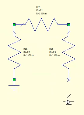
Step 19: Click to place the ground on the other resistor.
Creating Ports
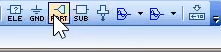
Step 20: Select the Port button from the toolbar.
Step 21: Click to place a port on the left terminal of the in-series resistor.
Step 22: Press CTRL-P on the keyboard to activate port placement.
Step 23: Press CTRL and right-click to flip the port horizontally.
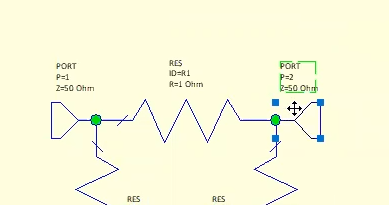
Step 24: Click to place the port on the other terminal of the in-series resistor.
Step 25: Press Home on the keyboard to enlarge the schematic as much as possible within the window boundary.
Defining Component Values
Step 26: Double-click the value of the series resistor to change it.
Step 27: Enter 10 for the value and click outside to set the value.
Step 28: Select one of the outer resistors, hold Shift, and select the other to select both.
Step 29: Double-click either value to open the Element Options window.
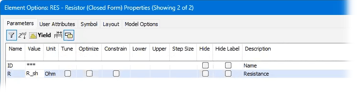
Step 30: Enter R_sh for the value.
Note: This will set the value of both shunt resistors to a variable.
Step 31: Click OK to save the settings and close the window.
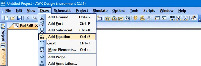
Step 32: Select Draw > Add Equation from the menu, the Add Equation button from the toolbar, or press CTRL-E on the keyboard.
Step 33: Click to place the equation in the canvas.
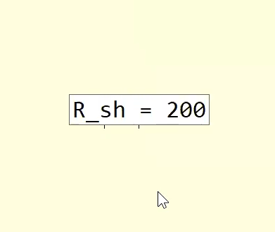
Step 34: Enter R_sh = 200 for the equation to define the shunt resistance as 200Ω.
Note: The variable name is case-sensitive. If entered incorrectly, the shunt resistor values are shown in red.
Creating a Graph
Step 35: Select the Add New Graph button from the toolbar. The New Graph window opens.
Step 36: Set the graph type to Rectangular.
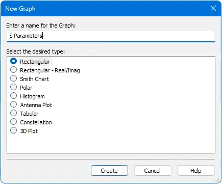
Step 37: Name the graph S Parameters and click Create. The graph opens in a new window.
Step 38: The windows can be organized to fill the entire workspace. Select the original Pad 3dB window to place it on the left.
Step 39: Select Window > Tile Vertical from the menu. The windows are arranged in a split screen configuration.
Note: With the schematic window selected, press Home on the keyboard to change the schematic view to show the entire circuit.
Adding Graph Data
Step 40: Right-click anywhere in the graph and select Add New Measurement.
Step 41: The Add Measurement window opens. Select Port Parameters as the Measurement Type if not already selected.
Step 42: Select S from the Measurement table.
Step 43: Set the To Port Index to 1.
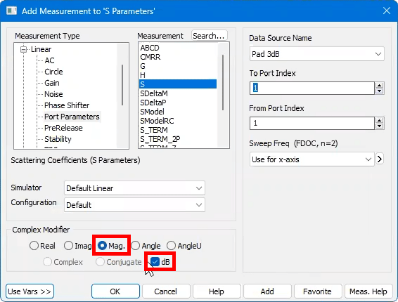
Step 44: Set the Complex Modifier to Mag. for Magnitude. Check dB.
Step 45: Select Add to add the plot.
Step 46: Set the To Port Index to 2 and click Add.
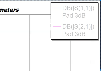
Note: A legend is created in the graph showing both plot functions.
Step 47: Click Close to close the Add Measurement window.
Running the Simulation
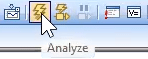
Step 48: Select the Analyze button from the toolbar to run the simulation.
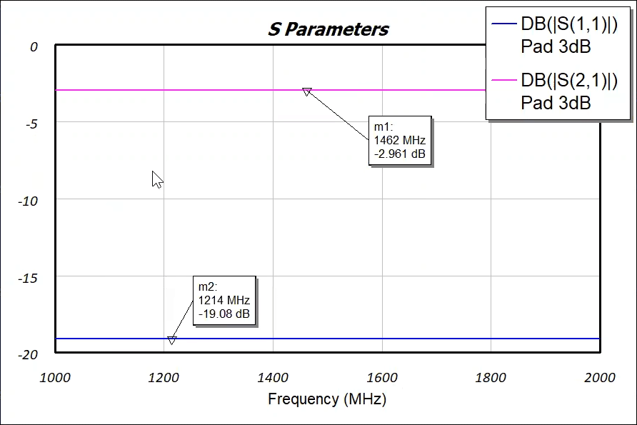
Step 49: View the results. The frequency-domain plots are flat, as expected.
Note: Click and drag the mouse on either trace to see the value at any point.
Step 50: Right-click in the graph and select Add Marker.
Step 51: Click to add a marker to the top plot. Click and drag to adjust the marker callout as needed.
Step 52: Right-click and select Add Marker. Click to add a marker to the bottom plot.
Configuring Parameters for Tuning
Step 53: Double-click the series resistor to add the tuning property.
Step 54: Check the Tune and Constrain cells in the options table.
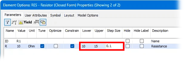
Step 55: Enter 10 into the Lower cell, 15 into the Upper cell, and 0.1 into the Step Size cell. Use the arrow keys to move between cells.
Step 56: Click OK to save the settings and close the window.
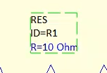
Note: The resistor value is now blue on the schematic, indicating that the value is tunable.
Step 57: Right-click the variable equation and select Properties.
Step 58: Under Tuning/Optimization, check Tune and Constrain.
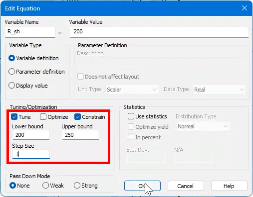
Step 59: Enter 200 for the Lower bound, 250 for the Upper bound, and 1 for the Step Size. Click OK.
Note: The variable text is now blue in the schematic, indicating that the value is tunable.
You can also use the Tune Tool button from the toolbar to make a variable or value tunable. This will only activate Tune. You will need to set the Constrain mode and boundaries manually.
Tuning the Components
Step 60: Select the Tune button from the toolbar. A set of sliders opens to adjust component values quickly.
Step 61: Click and drag the Tuner slider for the shunt resistor variable until the plotted value for S(1,1) is under -20dB.
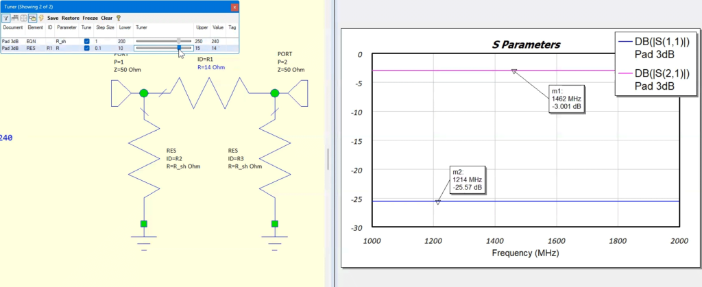
Step 62: Click and drag the Tuner slider for the series resistor until the plotted value for S(2,1) is -3dB.
Note: The graph updates automatically during tuning. Adjusting the value for either resistor will affect both plotted values. In this example, the shunt resistor values are 240Ω and the series resistor is 14Ω.
Step 63: Close the tuning window.
Wrap Up & Next Steps
Easily create and simulate an RF schematic for high-speed designs with AWR. Learn more about AWR and request a free trial here. For more AWR how-tos, visit EMA Academy.

