Achieving a robust and functioning power distribution network isn’t difficult, if we provide both the capacity and responsiveness needed at each device. Previous articles addressed capacity concerns, discussing the need for sufficient copper (or an alternative conductor) between a voltage source and any load depending on it for its supply. Today, we build on this and examine what’s required to maintain that network at a steady voltage. This will rely on sufficient “energy stores” and the conduction paths needed to deliver charge quickly to any location on the board experiencing “instantaneous demand”.
DC vs. AC (AKA Static vs. Transient)
Historically, nearly all power conversations pertaining to printed circuit boards have been lumped into two categories with the terms “Power DC” and “Power AC” emerging as almost standard terminology. Power DC is understandable as it addresses PDN capacity issues associated with inadequate copper.
Our experience with DC analysis revealed the simulation process, once thought to be complex, was nothing more than the visualization of Ohm’s law. With voltage defined in our DC supplies, and current by the operating requirements of each load, we found tools could readily calculate the resistance by extracting the geometry of the conductors. Utilizing these resistance models in conjunction with the current needs of each IC (defined by their electrical specifications) we found it easy to predict the DC voltage available in each chip given its distance from the source. This makes the cumulative resistance from the source the determining factor defining the DC performance each IC experienced.
The voltage loss observed during DC analysis is representative of the reductions we would expect when each device was drawing a continuous, unchanging current from its power source. This constant current, when drawn threw the resistive network of our PCB produce a voltage potential in the conductive path, reducing the realized value at the IC’s power pins. While this is infinitely valuable in establishing a base voltage, it does not, however, completely define the true conditions. This is where Power AC can help fill in the gaps.
Adding Time to the Equation
Power AC is not intuitive; it’s not actually alternating current under investigation, but rather transient or changing current. While admittedly a much more accurate representation of the situation, it still obscures the true objective. Our desired goal is to have no variants at all: steady, unwavering power rails at each voltage, true to the defined level despite varying demand. Ideally, this should be the condition seen by every dependent IC regardless of the distance from the source or the demands of its neighbors.
To be concise, we want no AC, transients, spikes, droops, dips, or deviations. Just rock-solid, steady voltage distribution networks capable of maintaining the voltage while responding to the instantaneous current demands of today’s high-speed devices. Power AC is all about eliminating voltage changes.
To fully validate our PDN we must look closer at the ACTUAL current present at the power pins of a load device. What we find is, while there is often a degree of continuous, steady current, there’s also bursts of current at varying frequencies. These bursts are the subject of “Transient Power Analysis,” often inaccurately referred to as “AC analysis”. With the new understanding that current can also vary over time and keeping our objective of “a steady minimum voltage at the load pins” in mind, we must reevaluate Ohms Law.
Ohms Law Redux
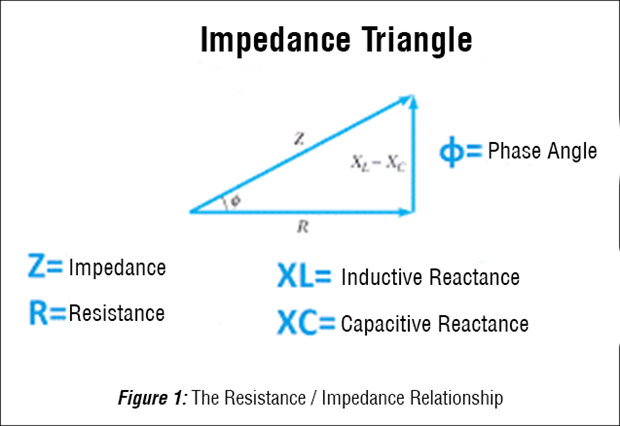
We must describe resistance using its complex definition: impedance. Impedance is simply the combination of resistance (R), which we know from DC analysis, and reactance. Reactance has both an inductive component, which resists changes in current, and a capacitive component which resists changes in voltage. In combination, they don’t reduce the voltage available at the load pins as we saw with DC losses, but rather they act to restrict or impede the responsiveness to the “burst demands” we described. With the effects of reactance altering the timing as opposed to the amplitude of a power signal we describe this behavior in terms of the effect on a sine wave, essentially advancing or retarding the signal and quantify it using degrees.
It All Comes Back to Impedance
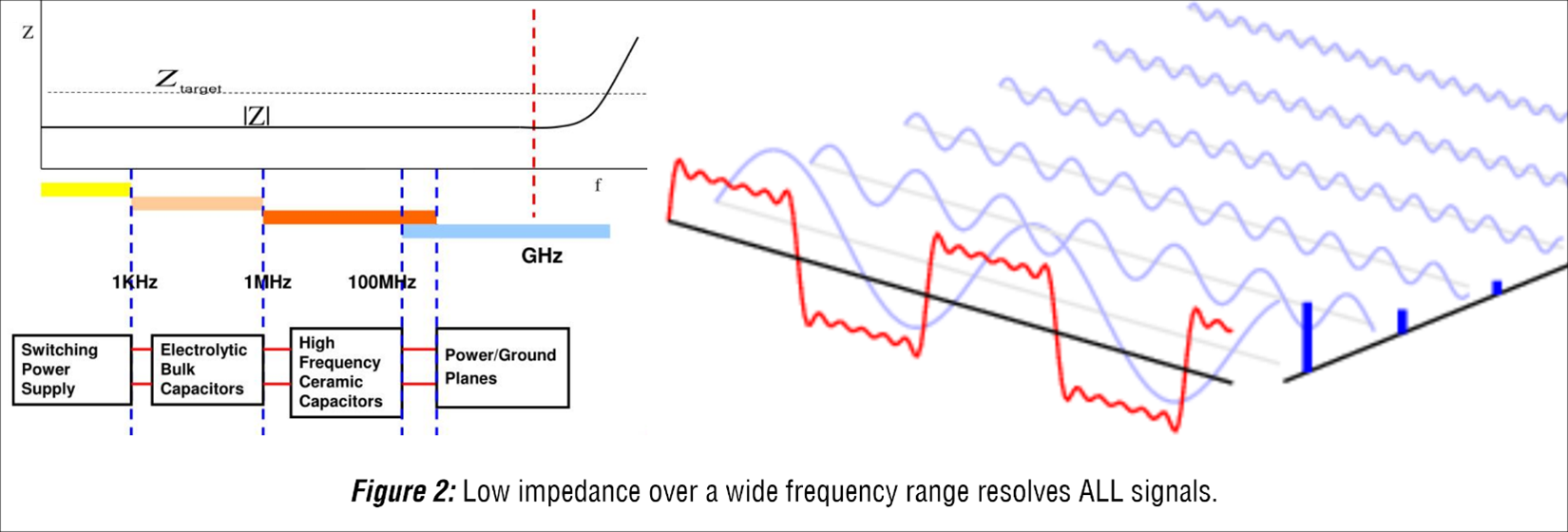
We now understand that to determine the ACTUAL voltage at the load pins, we must account for losses from both resistance and reactance. Comprised of both an inductive and a capacitive component, both influenced by frequency, we soon find the reactance (and therefore the impedance) changes with the frequency. Initially, this might suggest we would need to determine frequency before the resultant reactance could be known, however, in practice, we approach this a bit differently. With voltage our primary concern, and the knowledge that the loss of voltage results when the current (demanded by the load to operate) flows through the impedance of the PDN, it becomes clear that where Impedance stays low, the losses stay low. Therefore, our goal in PDN design is to maintain a low impedance over a range of frequencies, as opposed to just one. For example, maintaining an impedance at or below a specific goal (or “target”) for all frequencies between 1KHz and 1GHz will guarantee, via ohms law, the voltage loss will be at or below an acceptable loss without concern for the frequency associated with the reactance.
This “frequency range” approach has additional benefits as well. Using the mathematical process of transformation, we can represent any noise on the power plane as a combination of sine waves. As long as each sine wave is within the frequency range for low impedance, the resulting loss from the noise is limited. This essentially defines our design goals for the transient (aka “Power AC”) aspect of Power Integrity. Voltage is maintained indirectly by controlling the Impedance (frequency dependent resistance).
Controlling the Target Impedance
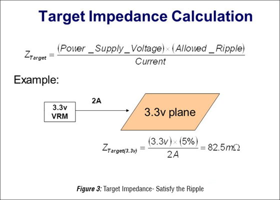
To some extent the terminology itself is confusing. Transient (or “AC”) Power Analysis isn’t about simulating the time-dependent noise on the power plane at all. Instead, it’s about ensuring the impedance is controlled. This way, any time-dependent variations in the current pass through a resistance so low it cannot produce a voltage high enough to be concerning. We control the variation in the voltage by limiting the resistance. Although each device has its own criteria for minimum voltage, as board designers, we determine how much variation we can allow in our supply voltage. Driven by the most demanding devices, acceptable “ripple”, or deviation from ideal voltage can be bounded simply by controlling the target impedance.
It All Becomes Clear… Once You Know the Answer
Our ability to meet a design’s requirements relies on our ability to control the resistance between a power source and each of its loads. It’s “partner”, inductance, represents the effects of changing current and replaces resistance with impedance in our calculation to include the reactance. The inclusion of reactance makes intuitive sense when we consider the two components from which it is constructed: inductance and capacitance. The goal of any PDN is to provide an adequate current at an unvarying voltage to every load. Therefore, it’s not hard to make the connection that a system with greater inductance, would be less capable of surging current-to-devices with varying requirements. Likewise, it’s not much of a stretch to see a system with high capacitance would be beneficial because of its resistance to voltage change.
While the mechanics of the physics involved is monumentally complex, with current traveling in all directions simultaneously and the signals themselves made from countless sinusoidal building blocks, the design goals are relatively modest. Reduce the resistance to minimize the DC loses and control the reactance by maintaining the impedance below the target over a wide range of frequency. In the real-world setting, where the current required by each device is dynamic (changing with time), the ability for a PDN to perform as intended is controlled exclusively by the systems impedance. Knowing this, the next question becomes: how do we use the techniques at our disposal to control it?
Continue reading this series to learn more about incorporating power delivery network analysis into your design process with Jernberg PI #5: The Case of the Noisy PDN.
Contact us for more information on how Sigrity can be used to analyze signal integrity and power integrity for PCB Designers.